

Robotic subsystems, embodiment and manipulator motion
- View
A laboratory arm must do more than reach
A laboratory robot transfers a specimen carrier from a loading station to an analytical instrument. Its gripper must approach the carrier, establish a secure grasp, transport it without striking the surrounding equipment, and present it at the correct orientation. A destination coordinate alone cannot specify this behaviour: the robot also requires a suitable mechanical structure, an executable movement and coordinated control.
This laboratory workcell provides the recurring scenario throughout the lesson. Its dimensions and operating conditions are illustrative engineering assumptions, not specifications for a commercial installation. The central question is practical: how do a robot’s constituent subsystems and physical embodiment determine the movements it can execute?
Robotic manipulation brings geometry, physical interaction and computation into a single engineering problem. MIT’s treatment of pick-and-place deliberately begins with geometry and kinematics even when object locations are assumed known, demonstrating that reliable movement remains a substantive problem independently of environmental perception. Understanding this foundation makes it possible to distinguish an inadequate movement model from an inadequate task specification. (manipulation.csail.mit.edu)
From a physical mechanism to a mathematical description
When the laboratory arm bends at its elbow, the attached forearm changes position; when its gripper closes, the fingers move relative to their supporting structure. These movements arise from links, the structural bodies of the mechanism, and joints, the connections that constrain their relative motion. A manipulator is a mechanism used to position and orient an end-effector, such as a gripper or an instrument. Kinematic models commonly treat links as rigid bodies, an approximation that makes their geometry tractable without representing every deformation. (motion.cs.illinois.edu)
| Comparison dimension | Revolute joint | Prismatic joint |
|---|---|---|
| Permitted movement | Rotation about an axis | Translation along an axis |
| Joint coordinate | An angle, normally expressed in radians | A displacement, normally expressed in metres |
| Illustrative workcell value | Elbow angle: (90^\circ=\pi/2) radians | Vertical slide displacement: (0.10) m |
These joint types each provide one independent motion coordinate. A robot’s degrees of freedom describe the number of independent coordinates required to specify its configuration, rather than the number of visible components or motors. For a fixed-base, open-chain arm with two independent revolute joints, the configuration is therefore (q=(q_1,q_2)), and the mechanism has two degrees of freedom. Additional constraints or mechanically coupled joints can invalidate a simple count of actuators. (motion.cs.illinois.edu)
Kinematics describes the geometric relationship between joint coordinates and the arrangement of the robot’s bodies. It does not, by itself, establish which forces or torques produce a movement. This distinction separates “the mechanism can occupy this arrangement” from “the mechanism can execute this movement under the specified load”. (motion.cs.illinois.edu)
Subsystems cooperate through feedback
The laboratory arm does not convert a task instruction directly into successful physical action. A movement reference must reach a controller, the controller must command the actuators, and the resulting configuration must be measured and compared with the reference. This relationship constitutes feedback control: commands are continually adjusted using information about the actual movement. Northwestern’s Modern Robotics describes this interaction as a stream of desired configurations, joint measurements and updated actuator commands. (modernrobotics.northwestern.edu)
For the illustrative workcell, consider an elbow reference of (90^\circ) and a measured angle of (87^\circ). Their difference is a (3^\circ) tracking error, not evidence that the specimen has reached its destination. A controller uses such discrepancies within its control law; the actuator and transmission produce the physical response. The mechanical assembly, power provision, measurement devices and computational components must therefore function as an integrated system, rather than as independently sufficient capabilities. The following allocation makes those responsibilities explicit. (roboticsbook.org)
| Subsystem responsibility | Contribution in the illustrative workcell | What it does not establish alone |
|---|---|---|
| Mechanical structure | Links, joints and mounting define the permitted geometry | Accurate execution under every load |
| Actuation and transmission | Drives produce and transmit joint effort | Knowledge of the achieved configuration |
| Power provision | Supplies energy to the drives and electronics | Correct movement commands |
| Measurement | Joint measurements support configuration feedback | Completion of the entire laboratory task |
| Computation and control | Generates references and updates actuator commands | Unlimited mechanical capability |
The useful engineering habit is to preserve these distinctions during diagnosis. In the (90^\circ/87^\circ) example, the discrepancy identifies a tracking issue that requires investigation; it does not uniquely identify its cause. A command is a requested outcome, not a measurement of an achieved outcome, and joint tracking alone does not certify successful object handling. (modernrobotics.northwestern.edu)
Embodiment makes the body part of the problem
Replacing the laboratory gripper with an elongated probe changes where contact occurs, even when every arm joint remains unchanged. The meaningful endpoint is now the probe tip rather than the former grasp centre. In this lesson, embodiment denotes the way the robot’s physical structure and attached tools condition its opportunities for action. Research on tool-as-embodiment explicitly treats tools as extensions of the manipulating body, rather than merely as interchangeable labels in a task description. (arxiv.org)
A precise embodiment model must identify the point and orientation relevant to the task. The tool centre point, or TCP, is the designated operational reference attached to the tool; it need not coincide with the wrist or mounting flange. In our illustrative workcell, attaching a rigid probe with its tip (0.12) m along the flange’s local forward axis introduces a corresponding geometric offset. The same flange pose then places the operational point somewhere different, so a tool change requires an updated geometric relationship rather than a renamed command. (manipulation.csail.mit.edu)
This relationship also clarifies the connection to metacognition without anthropomorphising ordinary control. METATOOL investigates computational models of synthetic awareness grounded in human metacognition and their validation through robotic experiments, including the broader problem of tool invention. That research ambition is not evidence that a conventional feedback controller possesses human-like awareness. Within this lesson, the defensible engineering principle is narrower: claims about action capability must refer to the robot’s actual body and attached tool, not an obsolete representation of them. (metatool-project.eu)
Joint configurations determine tool poses
An elbow angle describes one internal relationship, whereas a specimen-transfer instruction concerns an operational location and orientation. The complete set of permitted joint configurations forms the configuration space. A pose specifies position and orientation relative to a reference frame, and forward kinematics maps a configuration to the pose of a selected body or tool frame. Explicitly naming that reference frame prevents an otherwise ambiguous statement such as “move to (x=0.30) m”. (manipulation.csail.mit.edu)
The inverse question starts with a desired tool pose and seeks compatible joint configurations. This inverse kinematics problem may admit multiple solutions or none, depending on the mechanism and target. It is therefore mistaken to treat a tool coordinate as though it uniquely determines the arm’s posture. In a laboratory workcell, different compatible postures may place the elbow on different sides of surrounding apparatus, even when the operational endpoint is identical. (hades.mech.northwestern.edu)
| Comparison dimension | Joint-space description | Task-space description |
|---|---|---|
| Primary quantities | Joint angles or displacements | Operational position and, when required, orientation |
| Illustrative specification | (q_1=0^\circ,\ q_2=90^\circ) | Tool position (x=0.30) m, (y=0.20) m |
| Principal value | Specifies the mechanism’s configuration | Expresses the operational objective |
| Important limitation | Does not directly communicate the task outcome | May correspond to several configurations or none |
For the worked example below, the arm moves in a horizontal plane and has two revolute joints. Its idealised link lengths are (L_1=0.30) m and (L_2=0.20) m, with the TCP at the second link’s endpoint. These assumptions intentionally exclude vertical movement and independent tool-orientation control; the example describes planar positioning rather than a complete three-dimensional transfer system.
Worked example: positioning the specimen carrier
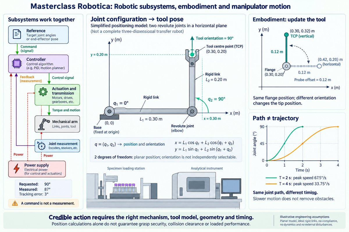
With the first link aligned along the base frame’s positive (x)-axis and the second link turned through (90^\circ), the endpoint lies (0.30) m forward and (0.20) m sideways. This geometric construction illustrates the forward-kinematics relationship without concealing it behind software. The following equations are derived for the stated two-link model, with the second joint angle measured relative to the first link.
[ x=L_1\cos q_1+L_2\cos(q_1+q_2) ]
[ y=L_1\sin q_1+L_2\sin(q_1+q_2) ]
- Specify the model: input (L_1=0.30) m and (L_2=0.20) m; output a defined two-link geometry.
- Specify the configuration: input (q_1=0^\circ) and (q_2=90^\circ); output absolute link directions of (0^\circ) and (90^\circ).
- Calculate the endpoint: input those lengths and directions; output (x=0.30) m and (y=0.20) m.
- Interpret the operational constraint: input the joint-angle sum; output a tool orientation of (90^\circ) relative to the base (x)-axis.
The result supplies both a position and an associated orientation; it does not provide independently selectable values for all three planar pose coordinates. This distinction matters when the carrier must enter a keyed instrument opening rather than merely arrive above a location. Within the wider laboratory workflow, the calculation supports compatibility checking between the mechanism and the instrument interface, but it does not establish grasp security, collision clearance or loaded tracking performance. MIT’s pick-and-place framework similarly distinguishes geometric representations from the additional requirements of executing manipulation. (manipulation.csail.mit.edu)
A destination is not a movement
Knowing the starting and finishing configurations leaves the intervening motion unspecified. A path describes a geometric sequence of configurations, while a trajectory associates that sequence with time. Time scaling determines how quickly the robot progresses along a path and consequently affects its velocity and acceleration requirements. Northwestern’s trajectory framework explicitly separates these two decisions, preventing “where to move” from being conflated with “how quickly to move”. (modernrobotics.northwestern.edu)
For an illustrative joint movement from (0^\circ) to (90^\circ), use the smooth interpolation (q(t)=90^\circ(3u^2-2u^3)), where (u=t/T). At (t=T/2), the joint reaches (45^\circ), regardless of the selected duration (T). Its peak speed is (135^\circ/T), giving the values below; these are mathematical results for the specified profile, not recommended operating speeds.
| Comparison dimension | Duration (T=2) s | Duration (T=4) s |
|---|---|---|
| Geometric joint path | (0^\circ) to (90^\circ) | (0^\circ) to (90^\circ) |
| Time at (45^\circ) | (1) s | (2) s |
| Peak joint speed | (67.5^\circ/\text{s}) | (33.75^\circ/\text{s}) |
The longer duration preserves the path while reducing this profile’s peak speed. It does not remove an obstruction intersecting that path, nor does smooth interpolation alone establish that the movement respects every actuator or loading constraint. A sound specification therefore distinguishes geometric validity, timing and physical execution instead of treating successful endpoint calculation as sufficient. (modernrobotics.northwestern.edu)
Worked example: exchanging the gripper for a probe
Where does the probe tip actually go?
The same laboratory workcell now uses a probe to operate a recessed instrument control. For this illustrative operation, the flange is at ((0.30,0.20)) m and the probe extends (0.12) m along its local forward axis. When that axis points along the base frame’s positive (x)-direction, the tip lies at ((0.42,0.20)) m; when it points along positive , the tip lies at ((0.30,0.32)) m. These values follow directly from rotating the tool offset into the base frame before adding it to the flange position.
- Define the attached tool: input a (0.12) m local forward offset; output the flange-to-tip geometric relationship.
- Apply the flange orientation: input a (90^\circ) orientation; output a base-frame offset of ((0,0.12)) m.
- Calculate the operational point: input flange position ((0.30,0.20)) m; output tip position ((0.30,0.32)) m.
- Specify the contact objective: input desired tip position ((0.30,0.32)) m at (90^\circ); output the corresponding flange pose for subsequent feasibility checking.
The benefit is operational precision: the workcell specification refers to the point that actually contacts the instrument. The limitation is equally important: accounting for the tip does not establish clearance for the probe shaft, wrist or arm. Updating a tool relationship therefore belongs within the wider configuration and movement-validation workflow, rather than being treated as a cosmetic change to the task name. This example applies the frame-based geometric reasoning used in robotic manipulation and the broader conception of tools as embodiment extensions. (manipulation.csail.mit.edu)
From coordinates to credible action
The laboratory scenario exposes four connected requirements: a coordinated robotic system, an explicit representation of its body, a geometric mapping between joints and operational poses, and a movement specification that includes time. None substitutes for the others. A credible manipulation claim identifies not merely a desired endpoint, but the mechanism, tool and executable movement to which that endpoint belongs. (roboticsbook.org)
-
Separate commands from achieved states: a requested configuration is not proof of physical arrival.
-
Represent the attached tool explicitly: the flange and operational point need not coincide.
-
Distinguish configuration from pose: the same task objective may admit different postures.
-
Distinguish path from trajectory: geometry and timing impose different requirements.
Next, we’ll build on this by exploring Sensing and environmental perception.